Deep Learning

Deep learning is a specialized subset of machine learning that uses multi-layered neural networks to analyze and process data, mimicking the way the human brain works. It is particularly effective at recognizing complex patterns and making decisions based on large amounts of unstructured data.

Tool/Framework	Description
Deepforge	A modern development environment for deep learning
Havorod	Distributed training framework for TensorFlow, Keras, PyTorch, and Apache MXNet
DeepSpeed	Deep learning optimization library

Neural Networks

Neural network consists of layers of interconnected nodes, or neurons, that collaborate to process input data. In a fully connected deep neural network, data flows through multiple layers, where each neuron performs nonlinear transformations, allowing the model to learn intricate representations of the data.

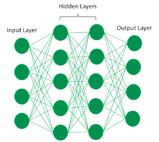
In a deep neural network, the input layer receives data, which passes through hidden layers that transform the data using nonlinear functions. The final output layer generates the model’s prediction.

• Input Layer: Receives raw data (e.g., pixels, words).
• Hidden Layers: Extract hierarchical features (shallow → deep layers).
• Output Layer: Produces predictions (e.g., class labels, regression values).

Activation Functions

In a neural network, activation functions are like the decision-makers. They determine what information should be passed along to the next layer. These functions add a level of complexity, enabling the network to learn from the data and make nuanced decisions. Introduce non-linearity to model complex patterns:

• ReLU (Rectified Linear Unit): Most common (fast, avoids vanishing gradients).
• Sigmoid/Tanh: For probabilities or bounded outputs.
• SoftMax: For multi-class classification.

Loss Function

The loss function is the difference between actual and predicted values. It allows neural networks to track the model’s overall performance. Depending on specific problems, we chose a certain type of function, for example:

• Mean Squared Error (MSE).
• Binary cross-entropy
• Categorical hinge
• Huber
• Sparse categorical cross-entropy

Backpropagation

In forwarding propagation, we initialize our neural network with random inputs to produce an output that is random too. To make our model perform better, we adjust weights randomly using backpropagation. To track the model’s performance, we need a loss function that will find global minimal to maximize the model’s accuracy.

Stochastic Gradient Descent

Gradient descent is used to optimize loss function by changing weights in a controlled way to achieve minimum loss. Now we have an objective, but we need direction on whether to increase or decrease the weights to achieve better performance. The derivative of the loss function will give us direction and we can use it to update the weights of the network.

An optimization algorithm used to minimize a loss function $J(\theta )$ by iteratively adjusting model parameters $\theta$

${\theta }_{t+1}={\theta }_t-\alpha \cdot \nabla J({\theta }_t)$ Where:

• ${\theta }_t$ = Current model parameters (weights, biases) at step $t$.
• $\alpha$ = Learning rate (step size, controls how aggressively we update $\theta$).
• $\nabla J({\theta }_t)$ = Gradient (vector of partial derivatives of $J$ w.r.t. each $\theta$).

Type	How It Works	When to Use
Batch GD	Computes gradient over the entire dataset per step.	Small datasets, precise updates.
Stochastic GD (SGD)	Uses one random sample per step (noisy, but faster).	Large datasets, escapes local minima.
Mini-Batch GD	Compromise: Uses small random subsets (batches) per step.	Most common (balances speed/accuracy).

Hyperparameter

Hyperparameters are the tunable parameters adjusted before running the training process. These parameters directly affect model performance and help you achieve faster global minima.

List of most used hyperparameters:

• Learning rate: step size of each iteration and can be set from 0.1 to 0.0001. In short, it determines the speed at which the model learns.
• Batch size: number of samples passed through a neural network at a time.
• Number of epochs: an iteration of how many times the model changes weights. Too many epochs can cause models to overfit and too few can cause models to underfit, so we have to choose a medium number.

Techniques

Various methods can be used to create strong deep learning models.

Learning rate decay

The learning rate is a hyperparameter - a factor that defines the system or sets conditions for its operation prior to the learning process - that controls how much change the model experiences in response to the estimated error every time the model weights are altered. Learning rates that are too high can result in unstable training processes or the learning of a suboptimal set of weights. Learning rates that are too small can produce a lengthy training process that has the potential to get stuck.

The learning rate decay method - also called learning rate annealing or adaptive learning rate - is the process of adapting the learning rate to increase performance and reduce training time. The easiest and most common adaptations of the learning rate during training include techniques to reduce the learning rate over time.

Common techniques in the learning rate decay method include the following:

• Step decay. Reduces the learning rate by a factor at specific intervals.
• Exponential decay. Continuously decreases the learning rate at an exponential rate.
• 1/t decay. Reduces the learning rate inversely proportional to the iteration number.

Transfer learning

This process involves perfecting a previously trained model on a new but related problem. It requires an interface to the internals of a preexisting network. First, users feed the existing network new data containing previously unknown classifications. Once adjustments are made to the network, new tasks can be performed with more specific categorizing abilities.

This method has the advantage of requiring much less data than others, thus reducing computation time to minutes or hours.

Training from scratch

This method requires a developer to collect a large, labeled data set and configure a network architecture that can learn the features and model. This technique is especially useful for new applications, as well as applications with many output categories. However, it’s a less common approach, as it requires inordinate amounts of data and computational resources, causing training to take days or weeks.

Dropout

This method attempts to solve the problem of overfitting in networks with large amounts of parameters by randomly dropping units and their connections from the neural network during training.

It has been proven that the dropout method can improve the performance of neural networks on supervised learning tasks in areas such as speech recognition, document classification and computational biology.

Neural Network Architectures

Standard

Perceptron

• The simplest type of neural network unit.
• Performs binary classification using a linear decision boundary.

Multilayer Perceptron (MLP)

• A feedforward neural network with one or more hidden layers.
• Can model non-linear functions using activation functions like ReLU, sigmoid, or tanh.

Residual Networks (ResNet)

ResNets provide an alternate pathway for data to flow to make the training process much faster and easier. The core idea behind ResNet is that a deeper network can be made from a shallow network by copying weight from the shallow counterparts using identity mapping.

The data from previous layers is fast-forwarded and copied much forward in the Neural Networks. This is what we call skip connections first introduced in Residual Networks to resolve vanishing gradients.

RNNs (Recurrent Neural Networks)

Recurrent Neural Network is a type of Artificial Neural Network that are good at modeling sequential data. Traditional Deep Neural Networks assume that inputs and outputs are independent of each other, the output of Recurrent Neural Networks depend on the prior elements within the sequence. They have an inherent “memory” as they take information from prior inputs to influence the current input and output. One can think of this as a hidden layer that remembers information through the passage of time.

Recurrent Neural Networks work very well with sequences of data as input. Its functionality can be seen in solving NLP problems like sentiment analysis, spam filters, time series problems like sales forecasting, stock market prediction, etc.

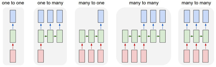
The input is in the form of sequential data that is fed into the RNN, which has a hidden internal state that gets updated every time it reads the following sequence of data in the input. Inputs-Outputs:

• One-to-one
• One-to-Many
• Many-to-one
• Many-to-many

LSTM (Long Short-term Memory Networks)

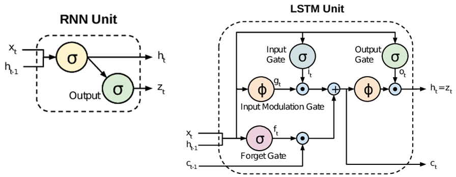
The critical part that we add to this Recurrent Neural Networks is memory. We want it to be able to remember what happened many timestamps ago. To achieve this, we need to add extra structures called gates to the artificial neural network structure.

CNNs (Convolutional Neural Networks)

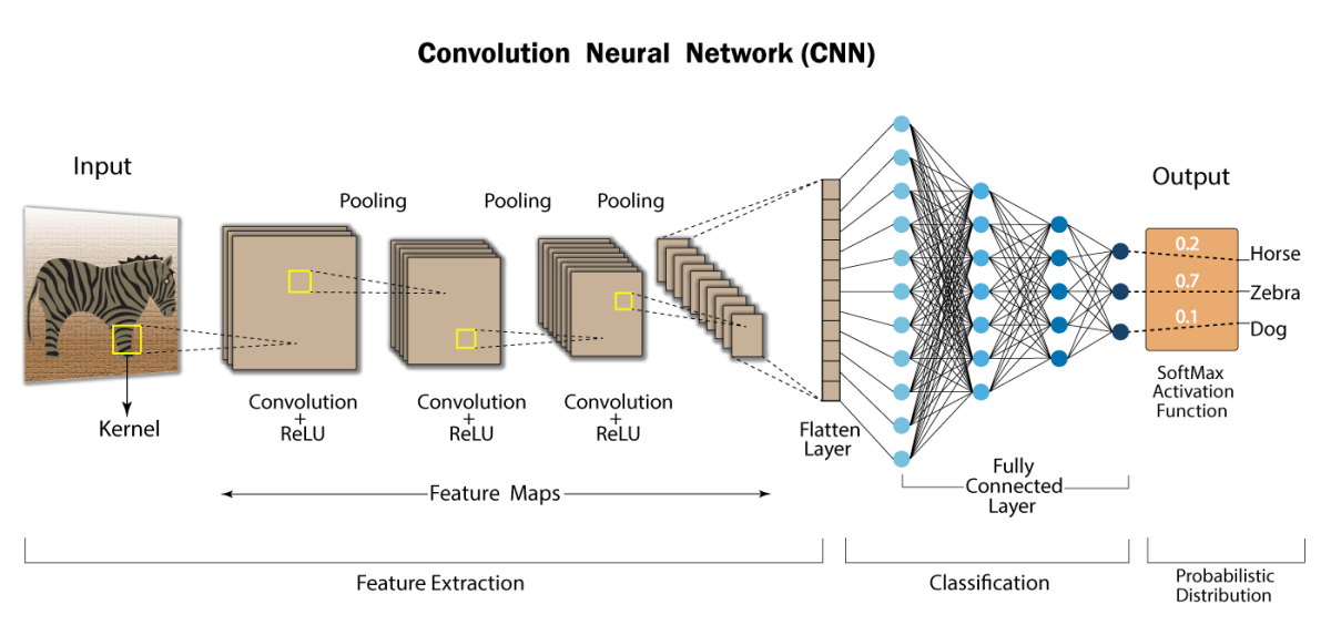
Convolution neural network (also known as ConvNet or CNN) is a type of feed-forward neural network used in tasks like image analysis, natural language processing, and other complex image classification problems.

Three hyperparameters that control the size of the output volume:

• The depth - The depth of the output volume is equal to the number of filters we use to look for different features in the image. The output volume has stacked activation/feature maps along with the depth, making it equal to the number of filters used.
• Stride - Stride refers to the number of pixels we slide while matching the filter with the input image patch. If the stride is one, we move the filters one pixel at a time. Higher the stride, smaller output volumes will be produced spatially.
• Zero-padding - It allows us to control the spatial size of the output volume by padding zeros around the border of the input data.

ReLU Layer

In this layer, the ReLU activation function is used, and every negative value in the output volume from the convolution layer is replaced with zero. This is done to prevent the values from summing up to zero.

Pooling

Pooling is a very important step in the ConvNets as it reduces the computation and makes the model tolerant towards distortions and variations. A Fully Connected Dense Neural Networks would use a flattened feature matrix and predict according to the use case.

Pooling layers are added in between two convolution layers with the sole purpose of reducing the spatial size of the image representation. Has two hyperparameters:

• window size
• stride

Types of Pooling:

• Max Pooling selects the maximum element from each of the windows of the feature map. Thus, after the max-pooling layer, the output would be a feature map containing the most dominant features of the previous feature map.
• Average Pooling computes the average of the elements present in the region of the feature map covered by the filter. It simply averages the features from the feature map.

Normalization layer

Normalization layers, as the name suggests, normalize the output of the previous layers. It is added in between the convolution and pooling layers, allowing every layer of the network to learn more independently and avoid overfitting the model.

CNNs Architectures

• LeNet
• AlexNet: was trained on the Imagenet dataset with 15 million high-resolution images with 256 * 256 * 3.
• MobileNets: use depth-wise separable convolutions to build lightweight deep Neural Networks
• VGGNet
• GoogLeNet
• SqueezeNet
• ResNet
• DenseNet
• ZFNet

DNNs (Deconvolutional Neural Networks)

Deconvolutional Neural Networks are CNNs that work in a reverse manner.

When we use convolutional layers and max-pooling, the size of the image is reduced. To go to the original size, we use upsampling and transpose convolutional layers. Upsampling does not have trainable parameters—it just repeats the rows and columns of the image data by its corresponding sizes.

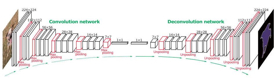
Transpose Convolutional layer means applying convolutional operation and upsampling at the same time. It is represented as Conv2DTranspose (number of filters, filter size, stride). If we set stride=1, we do not have any upsampling and receive an output of the same input size.

GANs (Generative adversarial networks)

A generative adversarial network (GAN), is a deep neural network framework that can learn from training data and generate new data with the same characteristics as the training data. For example, generative networks trained on photographs of human faces can generate realistic-looking faces which are entirely fictitious.

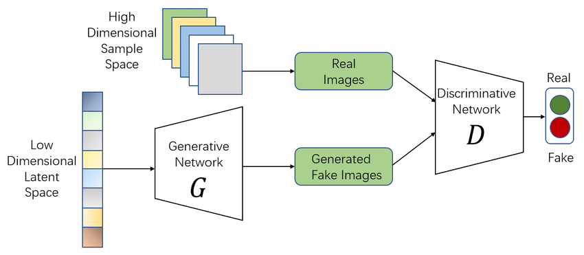
Generative adversarial networks consist of two neural networks, the generator, and the discriminator, which compete against each other. The generator is trained to produce fake data, and the discriminator is trained to distinguish the generator’s fake data from actual examples.

• Generator - The generator takes input as random noise and generates a data sample ideally in the latent space of the input dataset. Throughout the training, it tries to mimic the distribution of the input dataset.
• Discriminator - The discriminator network is a binary classifier that outputs whether the sample is real or fake. The input to the discriminator could either come from an input dataset or generator, and its task is to classify whether the sample is real or fake.

Examples:

• ‌Naïve Bayes
• Bayesian networks
• Markov random fields
• ‌Hidden Markov Models (HMMs)
• Latent Dirichlet Allocation (LDA)
• Generative Adversarial Networks (GANs)
• Autoregressive Model

Variants

DCGAN (Deep Convolutional GAN)

DCGAN is a generative adversarial network architecture based on CNNs. It uses a couple of guidelines, in particular:

• Replacing pooling layers with strided convolutions (discriminator) and fractional-strided convolutions (generator).
• Using batch norm in both the generator and the discriminator.
• Removing fully connected hidden layers for deeper architectures.
• Using ReLU activation in the generator for all layers except for the output, which uses tanh.

Progressive GANs

Generating high-resolution images is considered challenging for GAN models as the generator must learn how to output both overall structure and fine details simultaneously.

The primary contribution of the ProGan paper is a training methodology for GANs where we start with low-resolution images, and then progressively increase the resolution by adding layers to the networks.

Conditional GANs

A conditional generative adversarial network, or cGAN for short, is a type of GAN that involves the conditional generation of images by a generator model.

In cGANs, a conditional setting is applied, meaning that both the generator and discriminator are conditioned on some sort of auxiliary information (such as class labels or data) from other modalities.

Pix2Pix GAN

Pix2Pix is a Generative Adversarial Network, model designed for general-purpose image-to-image translation.

The image-to-image translation is the problem of changing a given image in a specific or controlled way. Examples include translating a landscape photograph from day to night or a segmented image to a photograph.

CycleGAN

The CycleGAN is a technique that involves the automatic training of image-to-image translation models without paired examples. The models are trained in an unsupervised manner using a collection of images from the source and target domain that do not need to be related in any way.

The CycleGAN is an extension of the GAN architecture that involves the simultaneous training of two generator models and two discriminator models.

• One generator takes images from the first domain as input and outputs images for the second domain. The other generator takes images from the second domain as input and generates images for the first domain.
• Discriminator models are then used to determine how plausible the generated images are and update the generator models accordingly.

Super-resolution GANs

Super-resolution (SR) upsampling a low-resolution image into a higher resolution with minimal information distortion. The generator network employs residual blocks, where the idea is to keep information from previous layers alive and allow the network to choose from more features adaptively.

DALLE-2

DALL·E 2 is a new AI system that can create realistic images and art from a description in natural language.

Algorithm explanation:

1. First, a text prompt is an input into a text encoder that is trained to map the prompt to a representation space.
2. Next, a prior model maps the text encoding to a corresponding image encoding that captures the semantic information of the prompt contained in the text encoding.
3. Finally, an image decoder stochastically generates an image which is a visual manifestation of this semantic information.