Machine Learning

Machine learning is a subfield of Artificial Intelligence that uses algorithms trained on data sets to create models that enable machines to perform tasks that would otherwise only be possible for humans, such as categorizing images, analyzing data, or predicting price fluctuations.

At its core, the method simply uses algorithms – essentially lists of rules – adjusted and refined using past data sets to make predictions and categorizations when confronted with new data. For example, a machine learning algorithm may be “trained” on a data set consisting of thousands of images of flowers that are labeled with each of their different flower types so that it can then correctly identify a flower in a new photograph based on the differentiating characteristics it learned from other pictures.

To ensure such algorithms work effectively, however, they must typically be refined many times until they accumulate a comprehensive list of instructions that allow them to function correctly. Algorithms that have been trained sufficiently eventually become machine learning models, which are essentially algorithms that have been trained to perform specific tasks like sorting images, predicting housing prices, or making chess moves. In some cases, algorithms are layered on top of each other to create complex networks that allow them to do increasingly complex, nuanced tasks like generating text and powering chatbots via a method known as “deep learning.”

Tool/Framework	Description
WebDataset	A high-performance Python-based I/O system for large
Lime	Explaining the predictions of any machine learning classifier
Elyra	Elyra extends JupyterLab with an AI centric approach
Autogoal	A Python framework for program synthesis with a focus on Automated Machine Learning
TorchScale	Transformers at any scale
Tiktoken	Fast BPE tokeniser for use with OpenAI’s models
Ray	Ray is a unified framework for scaling AI and Python applications
Aim	An easy-to-use & supercharged open-source experiment tracker
Meltano	The declarative code-first data integration engine that powers your wildest data and ML-powered product ideas
Hydra	Framework for elegantly configuring complex applications
Evidently	Evidently is an open-source ML and LLM observability framework.
LitServe	Lightning-fast serving engine for any AI model of any size

Articles/Talks

• Keeping your ML model in shape with Kafka, Airflow and MLFlow
• Introducing Elyra pipelines with custom component support
• Automate your machine learning workflow tasks using Elyra and Apache Airflow
• Elyra 3.3 - Pipelines, custom components, and catalogs
• Deploying ML Models in Production with FastAPI and Celery
• DiT - Self-supervised Pre-training for Document Image Transformer

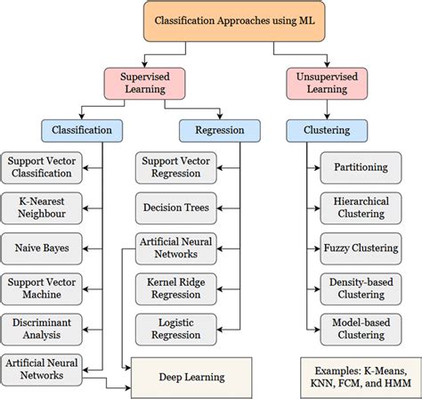
Supervised Learning

In supervised machine learning, algorithms are trained on labeled data sets that include tags describing each piece of data. In other words, the algorithms are fed data that includes an “answer key” describing how the data should be interpreted. For example, an algorithm may be fed images of flowers that include tags for each flower type so that it will be able to identify the flower better again when fed a new photograph.

Supervised machine learning is often used to create machine learning models used for prediction and classification purposes.

Classification

Binary Classification

• Predicts one of two possible classes (e.g., Yes/No, True/False, Spam/Not Spam).
• Algorithms used:
  • Logistic Regression
  • Support Vector Machines (SVM)
  • Decision Trees
  • Neural Networks
• Examples:
  • Email Spam Detection (Spam or Not Spam)
  • Medical Diagnosis (Disease or No Disease)
  • Fraud Detection (Fraudulent or Legitimate)

Multi-class Classification

• Predicts one class out of three or more possible classes.
• Algorithms used:
  • SoftMax Regression (Logistic Regression extended for multiple classes)
  • Random Forests
  • k-Nearest Neighbors (k-NN)
  • Neural Networks with multiple output neurons Examples:
• Handwritten Digit Recognition (0-9 digits)
• Animal Image Classification (Cat, Dog, Bird, etc.)
• Sentiment Analysis (Positive, Neutral, Negative)

Naive Bayes

Naive Bayes is a set of supervised learning algorithms used to create predictive models for binary or multi-classification tasks. It is based on Bayes’ Theorem and operates on conditional probabilities, which estimate the likelihood of a classification based on the combined factors while assuming independence between them.

Let’s consider a program that identifies plants using a Naive Bayes algorithm. The algorithm takes into account specific factors such as perceived size, color, and shape to categorize images of plants. Although each of these factors is considered independently, the algorithm combines them to assess the probability of an object being a particular plant.

Naive Bayes leverages the assumption of independence among the factors, which simplifies the calculations and allows the algorithm to work efficiently with large datasets. It is particularly well-suited for tasks like document classification, email spam filtering, sentiment analysis, and many other applications where the factors can be considered separately but still contribute to the overall classification.

Decision tree

A decision tree is a supervised learning algorithm used for classification and predictive modeling tasks. It resembles a flowchart, starting with a root node that asks a specific question about the data. Based on the answer, the data is directed down different branches to subsequent internal nodes, which ask further questions and guide the data to subsequent branches. This process continues until the data reaches an end node, also known as a leaf node, where no further branching occurs.

Decision tree algorithms are popular in machine learning because they can handle complex datasets with ease and simplicity. The algorithm’s structure makes it straightforward to understand and interpret the decision-making process. By asking a sequence of questions and following the corresponding branches, decision trees enable us to classify or predict outcomes based on the data’s characteristics.

This simplicity and interpretability make decision trees valuable for various applications in machine learning, especially when dealing with complex datasets.

Random forest

A random forest algorithm is an ensemble of decision trees used for classification and predictive modeling. Instead of relying on a single decision tree, a random forest combines the predictions from multiple decision trees to make more accurate predictions.

In a random forest, numerous decision tree algorithms (sometimes hundreds or even thousands) are individually trained using different random samples from the training dataset. This sampling method is called “bagging.” Each decision tree is trained independently on its respective random sample.

Once trained, the random forest takes the same data and feeds it into each decision tree. Each tree produces a prediction, and the random forest tallies the results. The most common prediction among all the decision trees is then selected as the final prediction for the dataset.

Random forests address a common issue called “overfitting” that can occur with individual decision trees. Overfitting happens when a decision tree becomes too closely aligned with its training data, making it less accurate when presented with new data.

K-nearest neighbor (KNN)

K-nearest neighbor (KNN) is a supervised learning algorithm commonly used for classification and predictive modeling tasks. The name “K-nearest neighbor” reflects the algorithm’s approach of classifying an output based on its proximity to other data points on a graph.

Let’s say we have a dataset with labeled points, some marked as blue and others as red. When we want to classify a new data point, KNN looks at its nearest neighbors in the graph. The “K” in KNN refers to the number of nearest neighbors considered. For example, if K is set to 5, the algorithm looks at the 5 closest points to the new data point.

Based on the majority of the labels among the K nearest neighbors, the algorithm assigns a classification to the new data point. For instance, if most of the nearest neighbors are blue points, the algorithm classifies the new point as belonging to the blue group.

Additionally, KNN can also be used for prediction tasks. Instead of assigning a class label, KNN can estimate the value of an unknown data point based on the average or median of its K nearest neighbors.

Support vector machine (SVM)

A support vector machine (SVM) is a supervised learning algorithm commonly used for classification and predictive modeling tasks. SVM algorithms are popular because they are reliable and can work well even with a small amount of data. SVM algorithms work by creating a decision boundary called a hyperplane. In two-dimensional space, this hyperplane is like a line that separates two sets of labeled data.

The goal of SVM is to find the best possible decision boundary by maximizing the margin between the two sets of labeled data. It looks for the widest gap or space between the classes. Any new data point that falls on either side of this decision boundary is classified based on the labels in the training dataset.

It’s important to note that hyperplanes can take on different shapes when plotted in three-dimensional space, allowing SVM to handle more complex patterns and relationships in the data.

Linear support vector classifier

A Linear SVC uses a boundary of one-degree (linear / straight line) to classify data. It has much less complexity than a non-linear classifier and is only appropriate for small datasets. More complex datasets will require a non linear classifier.

NuSVC

NuSVC uses Nu parameters which is for regularization. Nu is the upper bound on the expected classification error. If the value of Nu us 10% then 10% of the data will be misclassified.

Regression

Linear regression

Linear regression is a supervised machine learning technique used for predicting and forecasting values that fall within a continuous range, such as sales numbers or housing prices. It is a technique derived from statistics and is commonly used to establish a relationship between an input variable (X) and an output variable (Y) that can be represented by a straight line.

In simple terms, linear regression takes a set of data points with known input and output values and finds the line that best fits those points. This line, known as the “regression line,” serves as a predictive model. By using this line, we can estimate or predict the output value (Y) for a given input value (X).

Linear regression is primarily used for predictive modeling rather than categorization. It is useful when we want to understand how changes in the input variable affect the output variable. By analyzing the slope and intercept of the regression line, we can gain insights into the relationship between the variables and make predictions based on this understanding.

Logistic regression

Logistic regression, also known as “logit regression,” is a supervised learning algorithm primarily used for binary classification tasks. It is commonly employed when we want to determine whether an input belongs to one class or another, such as deciding whether an image is a cat or not a cat.

Logistic regression predicts the probability that an input can be categorized into a single primary class. However, in practice, it is commonly used to group outputs into two categories: the primary class and not the primary class. To accomplish this, logistic regression creates a threshold or boundary for binary classification. For example, any output value between 0 and 0.49 might be classified as one group, while values between 0.50 and 1.00 would be classified as the other group.

Consequently, logistic regression is typically used for binary categorization rather than predictive modeling. It enables us to assign input data to one of two classes based on the probability estimate and a defined threshold. This makes logistic regression a powerful tool for tasks such as image recognition, spam email detection, or medical diagnosis where we need to categorize data into distinct classes.

Unsupervised machine learning

Unsupervised machine learning uses unlabeled data sets to train algorithms. In this process, the algorithm is fed data that doesn’t include tags, which requires it to uncover patterns on its own without any outside guidance. For instance, an algorithm may be fed a large amount of unlabeled user data culled from a social media site in order to identify behavioral trends on the platform.

Unsupervised machine learning is often used by researchers and data scientists to identify patterns within large, unlabeled data sets quickly and efficiently.

Clustering

K-means

K-means is an unsupervised algorithm commonly used for clustering and pattern recognition tasks. It aims to group data points based on their proximity to one another. Similar to K-nearest neighbor (KNN), K-means clustering utilizes the concept of proximity to identify patterns in data.

Each of the clusters is defined by a centroid, a real or imaginary center point for the cluster. K-means is useful on large data sets, especially for clustering, though it can falter when handling outliers.

Clustering algorithms are particularly useful for large datasets and can provide insights into the inherent structure of the data by grouping similar points together. It has applications in various fields such as customer segmentation, image compression, and anomaly detection.

Dimensional Reduction

PCA

Principal Component Analysis (PCA) takes a large data set with many variables per observation and reduces them to a smaller set of summary indices. These indices retain most of the information in the original set of variables. Analysts refer to these new values as principal components.

Principal component analysis simplifies large data tables. With a vast sea of data, identifying the most important variables and finding patterns can be difficult. PCA’s simplification can help you visualize, analyze, and recognize patterns in your data more easily.

UMAP

Uniform Manifold Approximation and Projection (UMAP) is a manifold learning technique that aims to reduce the dimensionality of data while preserving its topological structure. It is particularly useful for visualizing high-dimensional datasets in a low-dimensional space, typically two or three dimensions. UMAP is often compared to t-SNE (t-distributed Stochastic Neighbor Embedding) due to its similar application in data visualization, but it offers several advantages, including better preservation of global data structure and faster computation times.

Semi-supervised machine learning

Semi-supervised machine learning uses both unlabeled and labeled data sets to train algorithms. Generally, during semi-supervised machine learning, algorithms are first fed a small amount of labeled data to help direct their development and then fed much larger quantities of unlabeled data to complete the model. For example, an algorithm may be fed a smaller quantity of labeled speech data and then trained on a much larger set of unlabeled speech data in order to create a machine learning model capable of speech recognition.

Semi-supervised machine learning is often employed to train algorithms for classification and prediction purposes in the event that large volumes of labeled data is unavailable.

Reinforcement learning

Reinforcement learning uses trial and error to train algorithms and create models. During the training process, algorithms operate in specific environments and then are provided with feedback following each outcome. Much like how a child learns, the algorithm slowly begins to acquire an understanding of its environment and begins to optimize actions to achieve particular outcomes. For instance, an algorithm may be optimized by playing successive games of chess, which allow it to learn from its past success and failures playing each game.

Feature Engineering

Feature Selection

The process of identifying the most important and relevant features from the dataset. It helps reduce dimensionality, improve model performance, and avoid overfitting.

Filter Methods

• Use statistical techniques to score each feature.
• Examples: Correlation coefficient, Chi-squared test, Mutual Information.
• Independent of any machine learning algorithm.

Wrapper Methods

• Use a model performance metric to evaluate feature subsets.
• Examples: Recursive Feature Elimination (RFE), Forward/Backward Selection.
• More accurate but computationally expensive.

Embedded Methods

• Feature selection is built into the algorithm.
• Examples: Lasso (L1) regularization, Decision Trees feature importance.
• Balance between filter and wrapper methods.

Feature Extraction

Create new features by transforming or combining existing ones, usually to reduce dimensionality or capture hidden structures.

• PCA (Principal Component Analysis) — creates orthogonal features.
• t-SNE or UMAP — nonlinear projection into fewer dimensions.
• Text vectorization — e.g., TF-IDF, Word2Vec for NLP.
• Fourier transforms for signal data.

Encoding Techniques

Convert categorical or textual data into numerical formats so models can process them.

• One-Hot for few classes
• Label for ordinals
• Embeddings for semantics

One-Hot Encoding

• Creates binary columns for each category.
• Works well for nominal data (no order).
• Can cause high dimensionality if many unique values.
• Example: “Color” (Red, Green, Blue) becomes:
  • Red = [1, 0, 0], Green = [0, 1, 0], Blue = [0, 0, 1].

Label Encoding

• Assigns each category a unique integer.
• Useful for ordinal categories (e.g., low, medium, high).
• Can introduce unintended order for nominal variables.
• How it works: Assigns each category a unique integer.
  • Example: “Size” (Small=1, Medium=2, Large=3).

Embeddings

• Map categories into dense, continuous vector space.
• Often learned during training (e.g., in NLP with Word2Vec or deep models).
• Efficient for high-cardinality or hierarchical categories.
• Example: Word embeddings (Word2Vec) where “king” → [0.2, -0.5, 0.7].

Feature Transformation

Apply mathematical operations to normalize, scale, or enrich data:

• Normalization & Standardization
• Log/Square Root transformations
• Binning (e.g., age into age groups)
• Polynomial features (e.g., x², x³)
• Interaction terms (e.g., feature1 × feature2)

Handling Missing Values

Techniques for dealing with NaNs or incomplete data, which can be crucial for preserving model quality:

• Deletion (row-wise or column-wise)
• Imputation (mean, median, mode, or model-based)
• Flags (adding binary columns indicating missingness)

Model Evaluation

Cross-Validation

A set of strategies used to evaluate a model by splitting the dataset into multiple training and validation subsets.

K-Fold Cross-Validation

• Data is split into K equal parts (folds).
• The model is trained on K-1 folds and validated on the remaining fold.
• Repeated K times, with each fold used as validation once.
• Final performance is the average across all K runs.

Stratified K-Fold

• Like K-Fold but maintains the class distribution in each fold (important for classification).

Leave-One-Out (LOO)

• Special case of K-Fold where K = number of samples.
• High computational cost, used for small datasets.

Holdout Method

• Simple train/test split.
• Fast but more variance depending on split.

Evaluation Metrics

These are the quantitative measures used to judge the model’s predictions.

Classification

Accuracy

• The ratio of correct predictions to total predictions.
• May be misleading in imbalanced datasets.

$Accuracy=\frac{TruePositives(TP)+TrueNegatives(TN)}{TP+TN+FP+FN}$

Precision

• Of all positive predictions, how many were actually positive?
• Important when false positives are costly.

$Precision=\frac{TruePositives(TP)}{TP+FalsePositives(FP)}$

Recall (Sensitivity)

• Of all actual positives, how many were predicted correctly?
• Important when false negatives are costly.

$Precision=\frac{TruePositives(TP)}{TP+FalseNegatives(FN)}$

F1 Score

• Harmonic mean of precision and recall.
• Balances both false positives and false negatives.

$F1Score=2\times \frac{Precision\times Recall}{Precision+Recall}$

ROC-AUC (Receiver Operating Characteristic – Area Under Curve)

• Measures the model’s ability to distinguish between classes.
• Comparing multiple models.
• ROC Curve: Plots True Positive Rate (Recall) vs. False Positive Rate (FPR).
• AUC: Area under ROC curve (1 = perfect, 0.5 = random guessing).

Confusion Matrix

• A 2x2 matrix for binary classification showing:
  • True Positives (TP)
  • False Positives (FP)
  • True Negatives (TN)
  • False Negatives (FN)

A table showing actual vs. predicted classifications (for Binary/Multi-class).

	Predicted: Positive	Predicted: Negative
Actual: Positive	True Positive (TP)	False Negative (FN)
Actual: Negative	False Positive (FP)	True Negative (TN)

Regression

Mean Squared Error (MSE)

• Average of squared differences between predicted and actual values.
• Penalizes large errors more than smaller ones.

$MSE=\frac{1}{n}{\sum }_{i=1}^n(y_i-\widehat{y_i}{)}^2$

Root Mean Squared Error (RMSE)

• Square root of MSE. Same units as target variable.
• More interpretable than MSE.

$RMSE=\sqrt{MSE}$

Mean Absolute Error (MAE)

• Average of absolute differences between predicted and actual values.
• Less sensitive to outliers than MSE.

$MAE=\frac{1}{n}{\sum }_{i=1}^n|y_i-\widehat{y_i}|$

R² Score (Coefficient of Determination)

• Measures the proportion of variance in the target explained by the model.
• *Interpretation:
  • 1 = Perfect fit.
  • 0 = No better than predicting the mean.
  • Negative = Worse than the mean baseline.

$R^2=1-\frac{\sum (y_i-\widehat{y_i}{)}^2}{\sum (y_i-\overline{y_i}{)}^2}$

Hyperparameter Tuning

This is the process of optimizing the model’s configuration settings to maximize performance.

• A Practical Introduction to Grid Search, Random Search, and Bayes Search

Grid Search

• Exhaustively tries every combination of specified hyperparameter values.

Random Search

• Samples a fixed number of parameter settings from a defined range.

Bayesian Optimization (advanced)

• Uses probabilistic models to find optimal parameters faster.

Bias-Variance Tradeoff

Understanding this tradeoff is key to balancing model complexity:

• High Bias (Underfitting):
  • Model is too simple.
  • Fails to capture the underlying trend.
• High Variance (Overfitting):
  • Model is too complex.
  • Performs well on training data but poorly on unseen data.

Frameworks

Notebooks

Computation notebooks have been used as electronic lab notebooks to document procedures, data, calculations, and findings. Jupyter notebooks provide an interactive computational environment for developing data science applications.

Jupyter notebooks combine software code, computational output, explanatory text, and rich content in a single document. Notebooks allow in-browser editing and execution of code and display computation results. A notebook is saved with an .ipynb extension. The Jupyter Notebook project supports dozens of programming languages, its name reflecting support for Julia (Ju), Python (Py), and R.

Scikit-learn

XGBoost

Gradient boosting

Gradient boosting algorithms employ an ensemble method, which means they create a series of “weak” models that are iteratively improved upon to form a strong predictive model. The iterative process gradually reduces the errors made by the models, leading to the generation of an optimal and accurate final model.

The algorithm starts with a simple, naive model that may make basic assumptions, such as classifying data based on whether it is above or below the mean. This initial model serves as a starting point.

In each iteration, the algorithm builds a new model that focuses on correcting the mistakes made by the previous models. It identifies the patterns or relationships that the previous models struggled to capture and incorporates them into the new model.

Gradient boosting is effective in handling complex problems and large datasets. It can capture intricate patterns and dependencies that may be missed by a single model. By combining the predictions from multiple models, gradient boosting produces a powerful predictive model.

Pytorch

• Some Techniques To Make Your PyTorch Models Train (Much) Faster
• Efficient PyTorch I/O library for Large Datasets, Many Files, Many GPUs